|
Copyright (c) 2010 ykuroda All right reserved. |
|
Copyright (c) 2010 ykuroda All right reserved. |
![]()
![]()
![]()
![]()
![]()
![]()
![]()
1)Non-linear Least Square Optimization
The non-linear least square algorithm used in SPANA is the Damping Gauss-Newton
method, which successively minimizes the square sum of errors (ss) between
the observed and theoretical values by using the correction vector,ΔP, for the parameter vectors ,P, adjusted by the damping factor α ( 0 < α ≦ 1 ).
P k+1 = P k + α ΔP
The conditions for convergence of the optimized parameters are as follows.
a) the decrease of ss < 0.001% of ss
b) the changes of parameters < 0.01% of the parameters
2) Convergence and Initial Guesses of Parameters
Since the non-linear least square method searches for the minimum of
ss assuming local linearity of its surface, the successive minimization
procedure starting from an inappropriate initial guess values of parameters
sometimes results in convergence into a local minimum before finding the
true one (Fig.1). For instance the appropriate initial guess values of
parameters for the 1:1 complex formation system are obtained as follows
by using the extrapolated ΔAdsmax, the sample concentration, [A]0, and the half titrant concentration, [B]1/2 (Fig.2),
Δεestimate 〜 ΔAdsMax/[A]0
K estimate 〜 1/[B]1/2
In the case that the appropriate optimized result is not obtained by the
standard procedure, the following alterations sometimes effective.
a) large changes of initial guess values of parameters
b) fixation of exponential parameter,
c) elimination of largely deviating data
d) change of "Damping factor" (standard initial value = 1)1
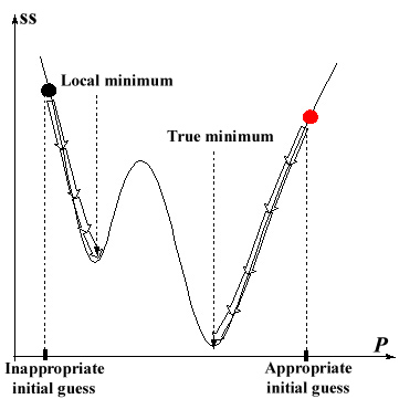 Fig.1
Fig.1 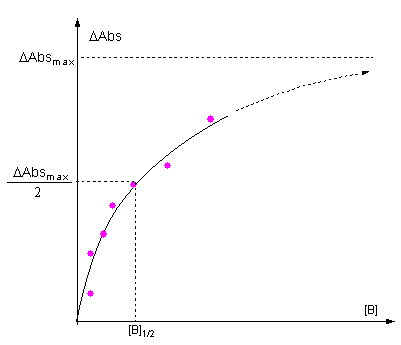 Fig.2
Fig.2
The extended Nelder-Mead Simplex method was added as an optimization calculation algorithm in SPANA Ver. 5.5.91. The Simplex method, which does not depend on local information of initial values, is slow to converge, but it has the potential to search a wider parameter space to find the global optimum value. This may be effective even in cases where only a very vague initial estimate parameters can be set due to the complexity of the system's computational model or the combination of a large number of parameters. An effective global search can be performed by repeating or combining the Damping Gauss-Newton and Nelder-Mead Simplex methods as appropriate for optimization while considering the speed of convergence and accuracy of the search.
3) Least Square Analyses of General Data 2
Since SPANA executes the least square optimization for the data (ti, Adsi) tabulated in the "Result" dialog box , the least square routine
of SPANA is applicable even for the general data in the table which are
not collected from SPANA. There are two methods for setting data in the
table;
a) call "Result" dialog box from the "Analysis-Least Square
Analyses-User' Data" menu
( defining the dimension of the table) and directly set the data into the cells by using
the numerical and arrow keys.
b) load the data from the data text file of the "*.lsq" format
(for the "*.lsq" format, see the manual)
For example, see Analyses of NMR Data and Concentration Data.
4) Non-linear Least Square Calculation for User's System (see also "Analysis"
and "Example")
SPANA ver.5 newly has the function of the non-linear least square analysis
for user's system which is not defined in SPANA. In order to link the user's
function to SPANA, two programs written in C language, spana_lsq.c (for
the usual non-linear least square analysis) and spana_redcap.c (for the
analysis of the reaction kinetics described in the form of differential
equations), are provided.. The user prepares the subroutine program defining
the theoretical model of user's system, which is compiled to generate the
executable program (*.exe)
For example, the least square analyses programs for NMR titration data
are provided as the archive file, "NMRTIT", in the "ExternalProgram.zip"
file (this function of the analysis of NMR titration data is practically
built in SPANA, see "Analysis of NMR Data").
a) General Non-linear Least Square Optimization (spana_lsq.c)
The subroutine program for spana_lsq.c describes the mathematical procedures
which calculates the theoretical values for the observed quantities, y[i].
The program written in C language is defined as "function(int i, double
x[], double p[])" and uses following four pre-declared array type
variables,
<< The Array Variables for "function" >>
y[j] : independent variable ( ex. ΔAbs in the spectroscopic titration),
j = 1-30
x[1] : dependent variables (ex. concentrations of the titrant), the
dimension is fixed to 1 for SPANA
c[k] : constants defining the system (ex. concentrations of the sample), k = 1-30
p[l] : parameters optimized, l = 1-100
The general form of the "function" subroutine is as follows,
#include <math.h>
external double y[],c[];
void function(int i, double x[], double p[])
{
(double ......; )
(int ......; )
/* define y[i] as functions of x[1], p[j], and c[k] here */
return;
}
The first three lines, #include <math.h> , external double y[],c[]、and
void function(int i, double x[], double p[]) are formulas to indicate that
this subroutine belongs to the main program, spana_lsq.c. The integer variable,
i, is used as the index identifying the individual y[i]. If other variables
are necessary, declare real variable as "double" and integer
ones as "int".
For example, preparations of the subroutine program for the following 1:
1: 1ternary complex formation system are shown below.
A + B <-> AB K1=[AB] / [A][B] eq.1
AB + C <-> ABC K2= [ABC] / [AB][C]eq.2
The solution of the spectroscopically active sample, A, is titrated with
mixture titrant of the transparent B and C. Then,
[A]0 = [A] + [AB] +[ABC] eq.3
[B]T = [B] + [AB] + 「ABC] eq.4
[C]T = [C] + [ABC] eq.5
where {A]0, [B]T and [C]T are the initial concentration of A (constant) and the total concentrations
of [B] and [C], respectively.
The different spectrum, ΔAbs, which is the subject for optimization is
ΔAbs = Abs - εA[A] 0 = Δε1[AB] + Δε2[ABC] eq.6
( Δε1= εAB - εA , Δε2= εABC - εA)
The values of [AB] and [ABC] are evaluated by solving the simultaneous
equations, eq.1-eq.5.
The following is one of the example of the calculation procedures, where
[B] is evaluated first.
Using eq.1, 2 and 5,
[C] = [C]T / ( 1 + K1K2[A][B] ) eq.7
and eq.3 is modified using eq.1, eq.2 and eq.7,
[A]0 = [A] + K1[A][B] + K1K2[C]T[A][B] / ( 1 + K1K2[A][B] ) eq.8
then, the following quadratic equation of [A] is obtained.
K1K2[B] ( 1 + K1[B] ) [A]2 + ( 1 + K1[B] ( 1 + K2 ([C]T -[A]0 ))) [A] - [A]0 = 0 eq.9
Simplifying the coefficients as shown below,
a = K1K2[B] ( 1 + K1[B] ) , b = ( 1 + K1[B] ( 1 + K2 ([C]T -[A]0 ))) , c = -[A]0
the solution, [A]B, as the function of [B] is
[A]B = (-b + (b2 - 4ac)1/2)/2a eq.10
then [C]B as the function of [B] is、
[C]B = [C]T / ( 1 + K1K2 [A]B[B] ) eq.11
Using [A]B、[C]B and eq.4, following eq.12 is obtained.
[B]T = [B] + K1[A]B[B] + K1K2[A]B[B][C]B eq.12
or
f ([B]) = [B] + K1[A]B[B] + K1K2[A]B[B][C]B - [B]T eq.13
[B] is the solution of f ([B]) = 0.
Since eq.13 has one solution in the area of 0 < [B] < [B]T for [B]T < [A]0 or [B]T - [A]0 < [B] < [B]T for [B]T > [A]0, the bisection method is used as most simple and widely applicable procedure for evaluation of [B] (for example of the bisection method, see http://en.wikipedia.org/wiki/Bisection_method).
Then, the values of [A] and [C] are evaluated from eq.10 and eq.7, respectively.
The example of the subroutine assuming [B]T = [C]T for the titrant and ΔAbs at five wave lengths is shown below,
/* Function for ABC Complexation Analysis */
/* A + B <---> AB K1= [AB]/[A][B] */
/* AB + C <---> ABC K2= [ABC]/[AB][C] */
/* Delta Abs = e1*[AB] + e2*[ABC] */
/* [A]0 = c[1], [C]T = [B]T = x[1] */
/* Delta Abs = y[i] (i = 1 - 5) */
/* K1 = p[1], K2 = p[2], */
/* e1 = p[3] - p[11], e2 = p[4] - p[12] */
#include <math.h>
extern double y[],c[];
double mfunction2(double h,double x[],double p[]);
void function(int i,double x[],double p[])
{
double max1,min1,mid,fl,fs,fm,af,bf,cf,ab,abc,aa,bb,cc;
int j;
if (x[1]==0) {ab=0;abc=0;goto org;} /* in case of [B]T = 0 */
max1=x[1]; /* start bisect algorism */
if (x[1]<c[1]) min1=0; else min1=x[1]-c[1];
fl=mfunction2(max1,x,p);fs=-x[1]; /* f([B]max) & f([B]min) */
if (fl*fs>0) goto fend1; /* goto rrror treatment */
for(j=1;j<=1000;j++) /* search [B] routine */
{
mid=(max1+min1)/2;fm=mfunction2(mid,x,p); /* f([B]mid) */
if (fm*fs>=0) min1=mid;
else
{if (fm*fl>=0) max1=mid; else goto fend1;}
if (fabs(fm)<1e-35) break; /* found [B] */
}
bf=mid; /* bf (free [B]) solution */
aa=p[1]*p[2]*bf*(1+p[1]*bf); /* coefficient aa */
bb=1+p[1]*bf*(1+p[2]*(x[1]-c[1]));cc=-c[1]; /* coefficient bb & cc */
af=(-bb+sqrt(bb*bb-4*aa*cc))/2/aa; /* af (free [A]) */
cf=x[1]/(1+p[1]*p[2]*af*bf); /* cf (free [C]) */
ab=p[1]*af*bf; /* ab ([AB]) */
abc=p[2]*ab*cf; /* abc ([ABC]) */
org:
switch (i)
{
case 1:
y[1]=p[3]*ab+p[4]*abc; /* Delta Abs = e1*[AB] + e2*[ABC] */
break;
case 2:
y[2]=p[5]*ab+p[6]*abc;
break;
case 3:
y[3]=p[7]*ab+p[8]*abc;
break;
case 4:
y[4]=p[9]*ab+p[10]*abc;
break;
case 5:
y[5]=p[11]*ab+p[12]*abc;
break;
}
return;
fend1:
printf("\nFail in finding the one root of function2");
}
double mfunction2(double h,double x[],double p[])
{
double f,af,cf,aa,bb,cc;
aa=p[1]*p[2]*h*(1+p[1]*h); /* bf=h */
bb=1+p[1]*h*(1+p[2]*(x[1]-c[1]));cc=-c[1];
af=(-bb+sqrt(bb*bb-4*aa*cc))/2/aa; /* af=[A] , eq.10 */
cf=x[1]/(1+p[1]*p[2]*af*h); /* cf=[C] */
f=h+p[1]*af*h+p[1]*p[2]*af*h*cf-x[1]; /* f([B])=[B]+[AB]+[ABC]-[B]o , eq.13 */
return (f);
}
The lines between /* and */ are comments. The values of ΔAbs at 5 wave
lengths are represented as y[1] - y[5], [B]T ( = [C]T) as x[1], [A]0 as c[1], K1 and K2 as p[1] and p[2], and Δε1、Δε2 at each wave length as p[3] - p[12].
Evaluation of f ([B]) is done in the new function, "double mfunction2(double h, double
x[], double p[])"
The executable program (*.exe) is obtained by linking and compiling these
source files, which can be carried out by usual commercial or free C compilers.
In the case of the free C compiler, DJGPP, or Microsoft Visual Studio C++, for example, the procedures are,
a) save the above source program as a text file, for example, "abc_comp.c"(
the extension "c" is recommended)
b) cmpile the source programs on the MS-DOS window, as follows,
"gcc -o abc_comp.exe spana_lsq.c abc_comp.c" for DJGPP, or
"cl abs_comp.c spana_lsq.c" for Visual Studio C++
This command make the executable program, "abc_comp.exe", which is able to be called from SPANA 3.
b) Least Square Program for Reaction Kinetics ( spana_redap.c )
The program, spana_redap.c, analyzes the data of the reaction trace, where
the theoretical model of the reaction system is described by the set of
the differential equations and the time-dependent theoretical values for
the observed trace are evaluated by the Runge-Kutta numerical integration
( for this numerical integration, see http://en.wikipedia.org/wiki/Runge%E2%80%93Kutta_methods).
Four following pre-declared variables are used for the standard subroutine
program, function(), for spana_redap.
<< The Array Variables for "function" >>
x[j] : variables for the observed data ( ex. concentration of chemical
species), i = 1-20
dx[i] : time differentials of x[i], i.e., dx[i]/dt
p[j] : parameters optimized, j = 1-30
c[k] : constants defining the system, k = 1-10
The general form of "function()" is shown below.
#include <math.h>
extern double dx[],x[],c[],p[];
void function()
{
/* define dx[i]/dt */
}
For example, the subroutine for the reaction, A -> B, catalyzed by C
is shown below.
k+ k2
A + C <->AC -> B + C eq.14
k-
This reaction is well known as Michaelis-Menten reaction under the conditions
of [A] >> [C] and the steady-state approximation. In the case that
these conditions are invalid, however, the reaction must be analyzed without
any simplification,
The full descriptions of the reaction in the differential forms are as
follows,
d[A]/dt = -k+[A][C] + k-[AC] eq.15
d[C]/dt = -k+[A][C] + (k- + k2)[AC] eq.16
d[AC]/dt = -(k- + k2)[AC] + k+[A][C] eq.17
d[B]/dt = k2[AC] eq.18
The subroutine is shown below,
/* Catalytic Reaction FOR REDAP */
/* A + C <-> AC -> B + C */
/* d[B]/dt = k[AC] */
/* p[1] = k+ , p[2] = k- , p[3] = k2 */
/* x[1] = [A] , x[2] = [B] , x[3] = [C] , x[4] = [AC] */
#include <math.h>
extern float dx[],x[],c[],p[];
void function()
{
dx[1]=-p[1]*x[1]*x[3]+p[2]*x[4];
dx[2]=p[3]*x[4];
dx[3]=-p[1]*x[1]*x[3]+(p[2]+p[3])*x[4]
dx[4]=-(p[2]+p[3])*x[4]+p[1]*x[1]*x[3];
}
void function2()
{
/* Define necessary equations to determined initial x[i] */
/* which is identified as '99999'. */
/* x[i]=g(x[j],p[i],c[i]) */
}
where [A], [B], [C], [AC], k+, k- and k2 are x[1], x[2]. x[3], x[4], p[1], p[2] and p[3], respectively..
Since the additional function, "void function2(), in this routine
is the reserved function which is not used here (used in the following
example), these lines are left as they are (don't erase).
The executable program (*.exe) is made by linking to spana_redap.c and
compiling with the C compiler.
c) Another Example for Kinetic Analysis
If k+, k- >> k2, the first step of eq.14 is able to be treated as the equilibrium process
K = [AC]/[A][C] eq.19
In this case, another version of the subroutine is derived as shown below.
Differentiation of eq.19 results in eq.20.
K[A]・d[C]/dt + K[C]・d[A]/dt = d[AC]/dt eq.20
Combining eq.20 with following kinetic relationships,
d[A]/dt + d[AC]/dt + d[B]/dt =0 eq.21
d[C]/dt + d[AC]/dt = 0 eq.22
d[B]/dt = k2[AC] eq.18
then the following set of differential equations is obtained.
d[A]/dt = -k2[AC] (1 + K[A])/(1 + K ([A] + [C])) eq.23
d[B]/dt = k2[AC] eq.24
d[AC]/dt = -k2K[C][AC]/(1 + K ([A] + [C])) eq.25
d[C]/dt = -d[AC]/dt eq.26
In this treatment, the initial concentrations of A, C and AC must be calculated
by the procedures for the equilibrium evaluation using the total concentrations
of A ([A]T = [A] + [AC] ) and C ([C]T = [C] + [AC] ) and eq.19 as follows,
[AC]initial = (K([A]T + [C]T) + 1 - ((K[A]T + [C]T + 1)2 - 4K2[A]T[C]T)1/2)/2K eq.27
[A]initial = [A]T - [AC] eq.28
[C]initial = [C]T - [AC] eq.29
These equations are defined as "function2()" in the subroutine.
Setting "99999" as the initial concentration in the execution
phase of the program, spana_redap uses this function2() to calculate these.
Although this kinetic system is equivalent to the Michaelis-Menten system,
this kinetic analysis procedures are applicable not only for the initial
reaction phase but also for the entire one.
The subroutine is shown below,
/* Michaelis-Menten Reaction FOR REDAP */
/* A + C <-> AC -> B + C */
/* K = [AC]/[A][C] */
/* d[B]/dt = k[AC] */
/* p[1] = K , p[2] = k */
/* x[1] = [A] , x[2] = [B] , x[3] = [C] , x[4] = [AC] */
/* c[1]= [A]o + [AC]o , c[2] = [C]o + [AC]o */
#include <math.h>
extern double dx[],x[],c[],p[];
void function() /* Definition of kinetic processes */
{
dx[1]=-p[2]*x[4]*(1+p[1]*x[1])/(1+p[1]*(x[1]+x[3]));
dx[2]=p[2]*x[4];
dx[3]=p[1]*p[2]*x[3]*x[4]/(1+p[1]*(x[1]+x[3]));
dx[4]=-dx[3];
}
void function2() /* Initial concentration for equilibrium process */
{
double tem;
tem=p[1]*(c[1]+c[2])+1;
x[4]=(tem-sqrt(tem*tem-4*p[1]*p[1]*c[1]*c[2]))/2/p[1];
x[1]=c[1]-x[4];
x[3]=c[2]-x[4];
}
where [A], [B], [C], [AC], K, k2, [A]T and [C]T are x[1], x[2]. x[3], x[4], p[1], p[2], c[1] and c[2], respectively..
In these programs shown above, the concentrations of the chemical species
are the subjects for evaluation. If the observed quantities are the indirect
data such as absorbance of the electronic spectra, the differential equations
for these observed quantities are necessary. For example, in the case that
the time dependency of the absorbance of electronic spectra, Abs, are the
data, the differential equation is
dAbs/dt = εAd[A]/dt + εACd[AC]/dt + εBd[B}/dt
where εA, εAC andεB are molar absorptivities for A, AC and B, respectively and this relationships
is defined in the subroutine as
dx[5]=p[3]*dx[1]+p[4]*dx[4]+p[5]*dx[2];
Note:
1) Usually, the initial value of the damping factor is 1 and, according to
the progress of optimization, the value is automatically adjusted. In the
case of analysis of badly non-linear system, a largely altered damping
factor is sometimes effective. The alteration is done in the dialog box of the least square calculation.
2) For more general non-linear least square optimization programs, LSPE and REDAP, are available, see Download page.
3) Because the DJGPP compiler is designed for the 32bit DOS, the "*.exe"
type program compiled by DJGPP does not run on the 64bit version of WINDOWS
7 or 8. For the 64bit compiler, for example, see the C++ compiler in Microsoft
Visual Studio.