SPANA for Spectral Data Analyses [Example] Copyright (c) 2010 ykuroda All right reserved. |
SPANA for Spectral Data Analyses [Example] Copyright (c) 2010 ykuroda All right reserved. |
![]()
![]()
![]()
![]()
![]()
![]()
![]()
Contents
1. Example of Equilibrium Analyses
2. Use of Multi-Titration Data
3. Titration by Spectroscopically Active Titrant
4. Analyses of Data Accompanying Dilution during Titration
5. Inverse Titration
6. Reduction of Number of Optimized Parameters (Fixation of Parameter Values)
7. Estimation of Spectra of Intermediates
8. Concentration of Chemical Species during Titration
9. Simulation
10. Wave Separation
11. Analyses of Multicomponent Spectra
12. 3D View
13. Analyses of NMR Data
14. Analyses of Concentration Data
15. Least Square Analyses for User's Function
1. Example of Equilibrium Analysis
a) Theoretical Model
The analysis of the simple sequential 1:2 complex formation
system, where the solution of A is titrated with B, is taken up as an example.
The equilibria are
A + B ↔ AB K1
= [AB]/[A][B] eq.1
AB + B ↔ BAB K2
= [BAB]/[AB][B] eq.2
and
[A]0 = [A] + [AB] + [BAB] eq.3
[B]0 = [B] + [AB] + 2[BAB] eq.4
Here, [A]0 is the initial (total) concentration of A and [B]0 is the total concentration of the titrant, B. If B is spectroscopically
transparent, the absorbance of the sample solution, Abs, is expressed as
Abs
= εA[A] + εAB[AB] + εBAB[BAB] eq.5
The difference spectra, ΔAbs, is obtained by using eq.3 and 5 as follow
ΔAbs
= Abs - εA[A] 0 = Δε1[AB] + Δε2[BAB] eq.6
where
Δε1= εAB - εA , Δε2= εBAB - εA
Since [AB] and [BAB] can be evaluated by using eq.1 - 4 with given K1,
K2, [A]0 and [B]0, the theoretically estimated ΔAbs is obtained from eq.6.
The least square calculation procedure determines the best parameter set,
K1, K2, Δε1, and Δε2, to minimize the following residual square sum, ss, resulting the best
fitting between the theoretical difference spectra, ΔAbs, and the observed
ones, ΔAbsobs.
ss
= Σ(ΔAbs - ΔAbsobs)2.
b) Analysis of Titration Data
The titration is usually performed under the condition
of [A]0 = constant during the experiment. According to eq.6, the values of ΔAbsobs are directly obtained by subtracting the initial spectra,εA[A] 0 ([B]0 = 0), from the observed titration spectra.
The practical procedures of the analyses of following spectral data set (Nondilute1-2_example.ana) are described below.
| [A]0=1x10⁻⁵ (M) | Spectrum00 | Spectrum01 | Spectrum02 | Spectrum03 | Spectrum04 | Spectrum05 | Spectrum06 | Spectrum07 |
| [B]0 (M) | 0 | 8.0x10⁻⁶ | 1.6x10⁻⁵ | 2.8x10⁻⁵ | 5.2x10⁻⁵ | 7.0x10⁻⁵ | 1.0x10⁻⁴ | 1.5x10⁻⁴ |
| Spectrum08 | Spectrum09 | Spectrum10 | Spectrum11 | Spectrum12 | Spectrum13 | Spectrum14 | Spectrum15 | |
| [B]0 (M) | 1.9x10⁻⁴ | 2.8x10⁻⁴ | 3.6x10⁻⁴ | 4.7x10⁻⁴ | 6.4x10⁻⁴ | 8.8x10⁻⁴ | 1.17x10⁻³ | 1.73x10⁻³ |
First, these 16 spectra are read and displayed on the screen of SPANA ("View-Activate All" menu or "click on Ch.0" and "shift + click on Ch.15") (Fig.1),
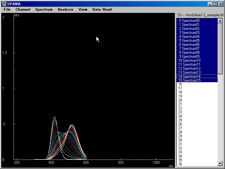
Fig.1 Spectra of original data
the display area is adjusted by using the "Format" dialog box ("View-Format" menu) (in this case, the "Auto Format" box is checked) (Fig.2),
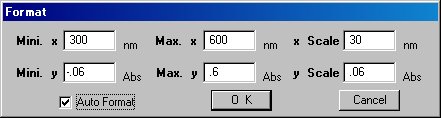 Fig.2
Fig.2
to display all spectra on the full screen (Fig.3).
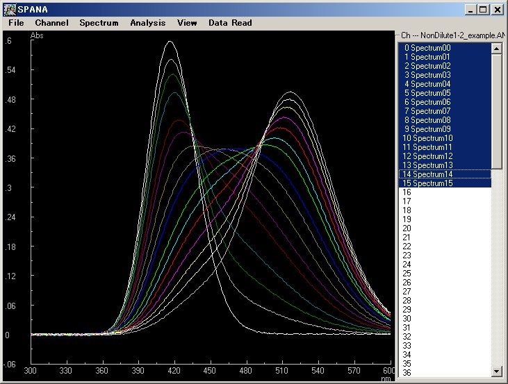 Fig. 3 Expanded original spectra
Then, the concentrations, [B]0, for each spectrum are inputted in the "Condition ( t )" items in the "Item Change" dialog box ("Channel-Item Edit" menu) (Fig.4),
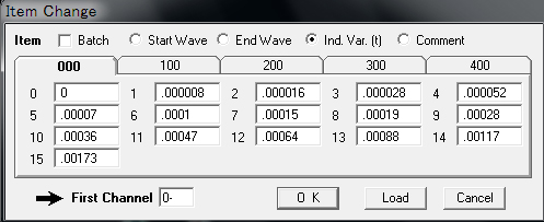 Fig.4
Fig.4
and the resultant spectra are overwritten on channel 0 -15 by assigning "0-" for "First Channel", where the hyphen, "-", is a keyword for successive writing (the channel names are automatically changed into Ch.0' and so on) (Fig.5).
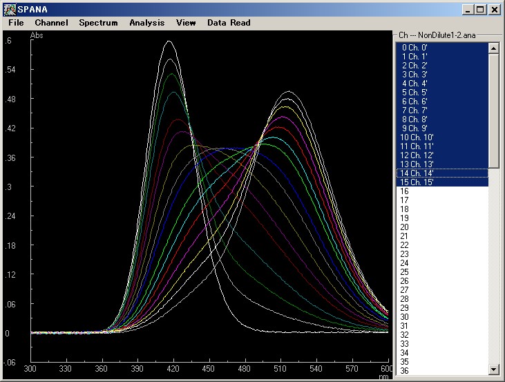 Fig.5 Setting of concentration
Before making ΔAbsobs, the 0-base lines of the spectra should be corrected by using the "Spectrum-Base Line-Average Correction" function assigning the area of 300 - 330 nm with shown vertical line-cursor (Fig.7).
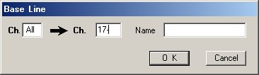 Fig.6
Fig.6
The resultant spectra are stored in the Channel 17 - 32 by setting "17-" as the target channels in the "Base Line" dialog box. (Fig.6).
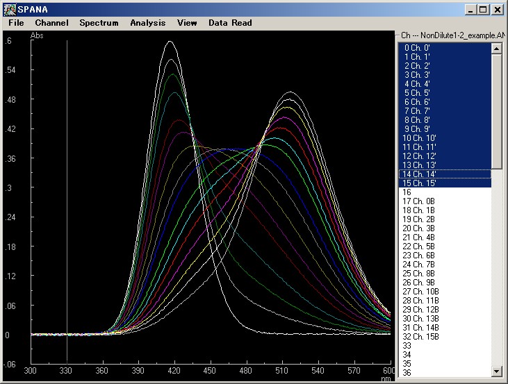
Fig.7 Base-line correction between 300-330 nm
The base-line corrected spectra are displayed by clearing the original spectra ("View-Deactivate All/Cls" menu) and activating (displaying) channel 17-32 by clicking on channel 17 and shift-clicking on channel 32 (selection of all channel between Channel 17 and 32) (Fig.8).
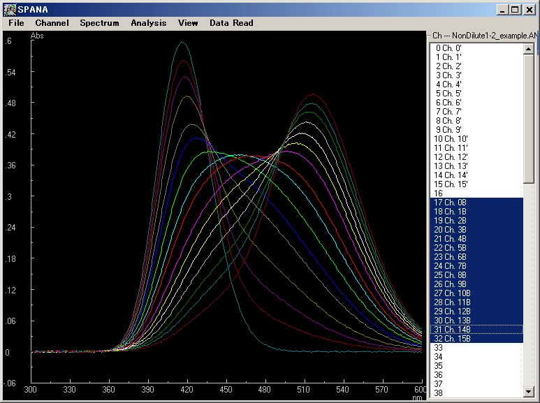 Fig.8 Base-line corrected spectra
Then, in order to making the ΔAbsobs spectra, the conditions for the subtraction are set in the "Data Edit" dialog box ("Spectrum-"-"-Channel" menu), i.e., Ch. "All" for the target spectra, the subtracter, εA[A] 0, channel (Ch."17"), and the channels which store the resulting difference spectra (Ch."34-") (Fig.9),
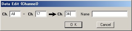 Fig.9
Fig.9
where "All" is a keyword meaning all active spectra and the resulting spectra are stored in successive Ch.34-49. The resulting difference spectra are shown as below (by changing the display status and format) (Fig.10).
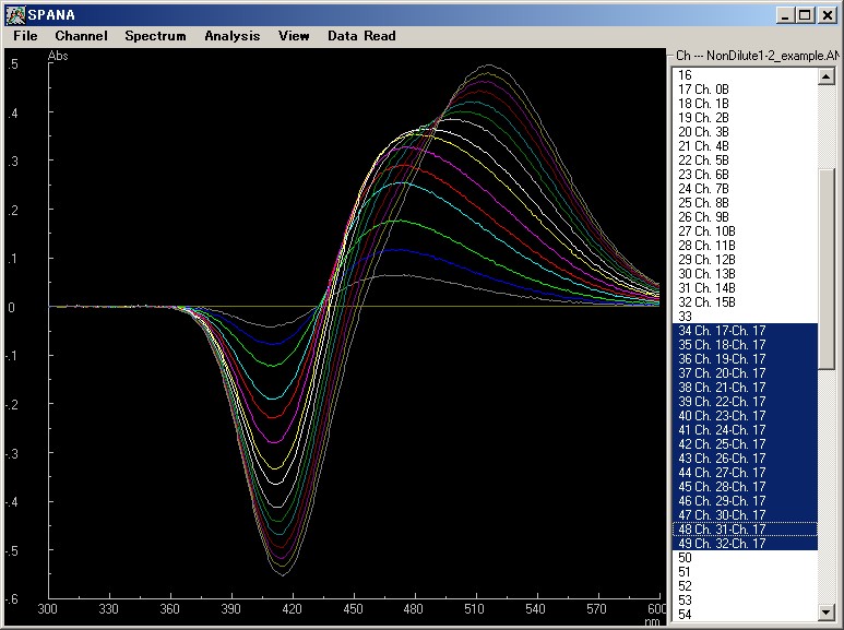 Fig.10 Difference spectra
Then, the sampling points for the least square calculation are collected by the cursor operation ("Analyses-Least Square Analyses-Point Data" menu) (Fig.11),
 Fig.11 Data sampling at 415, 450 and 516nm
where the data are sampled at 415nm (single click), 450nm (single click) and 516nm (double click for the final point) . In the cursor operations for data sampling, "single-click" at an arbitrary position is used for successive sampling and "double-click" for the final sampling to show the table of collected data in the "Result" table (Fig.12).*
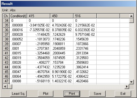 Fig.12
Click of the "Least Sq." button shows the "Least Square Analyses" dialog box to select the appropriate model for optimization (Fig.13).
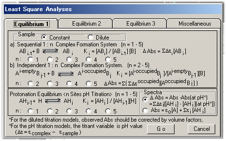 Fig.13
In this case, select "Sample : Constant" , and "Sequential 1 : n Complex Formation System - n : 2" in the page of Equilibrium Models 1, and click the "Go" button to show the "Least Square Optimization" dialog box (Fig.14).
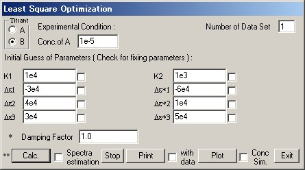 Fig.14
The dialog box shows the parameters to be optimized, K1, K2, Δε1, Δε2 (shown as Δε*1) at 415nm, Δε1, Δε2(Δε*2) at 450nm, Δε1, Δε2(Δε*3) at 516nm. Set the concentration A and initial guess values for the parameters and click the "Calc." button to start calculation.
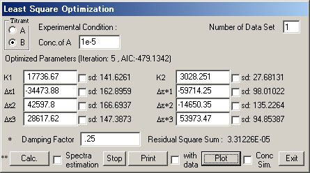 Fig.15
The final optimized parameters are shown in the dialog box together with
their standard deviations (sd) and the final residual square sum, ss (Fig.15).
In order to show the results graphically, click the "Plot" button
to show the "Graph Format" dialog box (Fig.16).
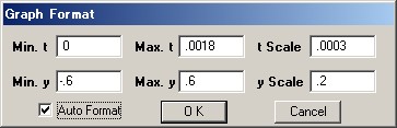 Fig.16
Check the "Auto Format" box and click "OK" button, then the graph plotting the observed data and the theoretical curves is shown as below (Fig.17).
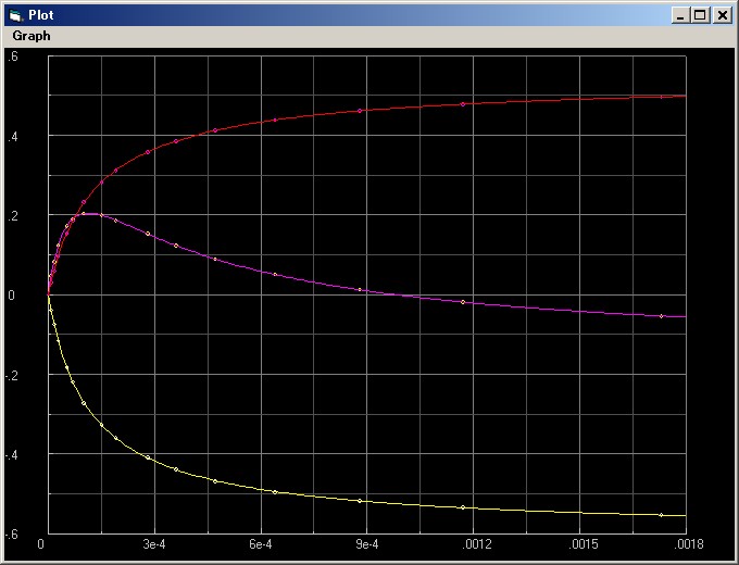
Fig.17 Plotting graph of [B]0 vs. observed data and titration curves at 516nm (red), at 450nm (purple)
and at 415nm (yellow)
* It should be noted that the reliability of the results is significantly depend on the data extraction and the model selection. For the example shown here, if the data at ~520nm changing monotonously are employed for analyses, the simple 1:1 complex formation model gives good fitting too.
2. Use of Multi-Titration Data
Data sampling at multi-wave length is effective in obtaining
statistically accurate results. Another more effective procedure is use
of multi-titration data which are collected from the independent titration
experiments. For example, SPANA can analyzes the data collected from the
titration experiments at the different [A]0 all together, which are arranged as data blocks separated by, at least,
one blank channel as shown below for the data in "Nodilute1-1-multi.ana" file containing the following data sets (Fig.18).
Set
1 : Ch. 15 - 24 ( [A]0 = 2 x 10⁻⁵ M )
Set
2 : Ch. 28 - 38 ( [A]0 = 1 x 10⁻⁵ M )
Set
3 : Ch. 42 - 51 ( [A]0 = 5 x 10⁻⁶ M )
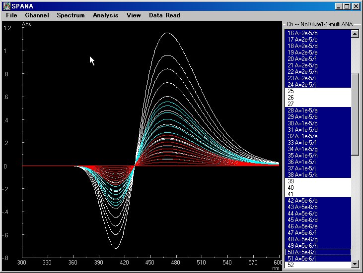
Fig.18 Spectra of data set 1 (white), 2 (light blue) and 3 (red).
The different points than the standard procedures for analyses of the single data set is that of calculation setting, i.e., after sampling the data and selecting the theoretical model, set "Number of Data Set = 3" in the "Least Square Optimization" dialog box, and, then, the additional information, the first channel and [A]0 value for each data set (Fig.19).
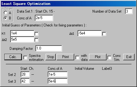 Fig.19
3. Titration by Spectroscopically Active Titrant
In the spectroscopic titration, the spectroscopically inactive (transparent) titrant is usually chosen, because the spectroscopically active titrant results in complex spectrum transformation due to overlapping of the effects of complex formation and titrant addition. However, if the absorbances of the titrant are so small that the Lambert-Beer's low is applicable during the experiment, the spectroscopic data are correctable for the extra absorbances of the titrant.
In such case, the observed absorbance, Abs, for the 1:2 complexation system
is
Abs
= εA[A] + εB[B] + εAB[AB] + εBAB[BAB] eq.5'
and the difference spectrum is
ΔAbs' = Abs - εA[A] 0 -εB[B] 0= Δε1[AB] + Δε2[BAB] eq.6'
where
Δε1= εAB - εA - εB , Δε2= εBAB - εA - 2εB
The values of εB[B] 0 are not constant and must be evaluated for each titration data, independently.
However, since the careful experiment make it possible to evaluate the
εB[B] 0 in SPANA, experimentally or calculably (by, for example, using standard
spectrum of a known concentration), the optimization analyses become possible
by using eq.6' which has the same form as eq.6.
4. Analyses of Data Accompanying Dilution during Titration
Usually, the concentration of the titrated sample, [A]0, must be kept constant during titration to obtain meaningful results.
The experimental procedures, however, are sometimes troublesome and wasteful
of the samples. If the Lambert-Beer's low is true during the experiment,
the spectroscopic data which accompany sample dilution caused by addition
of the titrant solution are correctable without losing accuracy.
For example, the theoretical model of the 1:2 complexation
model shown above is modified as follows,
[A]0 = (V/(V + v)) [A]org = [A] + [AB] + [BAB] eq.3'
[B]0 = (v/(V + v)) [B]org = [B] + [AB] + 2[BAB] eq.4'
where [A]org, [B]org , V, and v are the original concentrations of A, B, the initial volume
of A, and the added volume of the titrant, B, respectively. Then, the difference
spectra are modified,
ΔAbsdil = ((V + v)/V) Abs - εA[A]org
=
((V + v)/V) (Δε1[AB] + Δε2[BAB] ) eq.6'
Thus, the difference spectra, ΔAbsdil, made by subtraction of the initial spectrum, εA[A]org, from the observed titration spectra modified by the factor of (V + v)/V can be analyzed by the least square optimization as the "ΔAbsdil vs. v" system. SPANA has the special function which modifies the
data in this manner by using the "Concentration Correction" dialog
box (the "Spectrum-Conc.Correct" menu) (Fig.20).
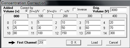 Fig.20
In this example, the modified spectra, ((V + v)/V) Abs, are calculated
for original observed spectra in Ch. 0-14 by using V=3000μL and v=0-300μL,
and stored in "Ch.20 -" .
Thus, making ΔAbsdil, selecting an appropriate "Diluted" model (for example, "1:2
Complexation System-Sequential Eq.-Diluted") in the "Least Square
Analyses" dialog box and setting the necessary parameters, [A]org, [B]org, and V, required in the "Least Square Optimization" dialog box
(Fig.21), the optimization is performed for the "ΔAbsdil vs. v" system to give the equilibrium constants and difference molar
extinction coefficients.
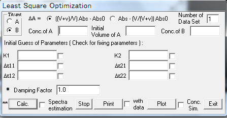 Fig.21
5. Inverse Titration
For the titration of 1 : n (A : B) multi-complex formation
system, B is often chosen as the titrant, because the normal saturation
behavior, formation of the 1 : n complex at the infinite concentration
of the titrant, is expected. In the case of the combination of spectroscopically
transparent A and avtive B, the titration experiment using A as the titrant,
however, is also possible, though the saturation at the infinite concentration
of the titrant means formation of the 1 : 1 complex. For the analyses of
such titration, change the titrant species (A) in the "Least Square
Optimization" dialog box (Fig.22).
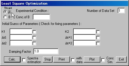 Fig.22
6. Reduction of Number of Optimized Parameters (Fixation of Parameter Values)
In the least square calculation optimizing many parameters, there may be the difficulty that the calculation can find no appropriate converging point for the best fitting and/or falls into a local minimum of ss. If some parameters are determinable by other experiments, there is a chance that these difficulties are avoided by fixing the known parameter values.
Checking the check box beside the parameter display area,
the parameter is treated as the constant and removed from optimization
calculation (see Fig.22).
7. Estimation of Spectra of Intermediates
SPANA has the function for estimating the intermediary
spectra which are not directly observed. The "Calc." operation
with check of the "Spectra estimation" check box in the "Least
Square Optimization" dialog box shows the "Estimated Spectra"
dialog box (Fig.23) after optimization
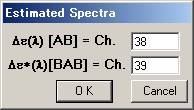 Fig.23
For the present sequential 1:2 complex formation system, the estimated difference spectra for AB and BAB are calculated and stored in the assigned channels. The spectra of AB and BAB are obtained by adding the initial spectrum, εA[A] 0, to the resulting difference spectra.
8. Concentration of Chemical Species during Titration
The "Plot" operation with check of the
"Conc. Sim." box shows the concentration of the chemical species
existing in the system during titration graphically. In the case of the
present sequential 1 : 2 complex formation system, the graph of [A], [B],
[AB], and [BAB] vs. [B]0 are prepared (Fig.24).
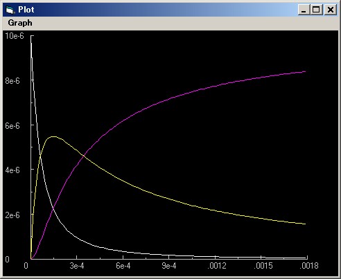
Fig.24 Concentration variations of [A] (white), [AB] (yellow) and [BAB]
(purple).
[B] is not shown graphically because of its too high concentration.
9. Simulation
The "Plot" operation in the "Least Square Optimization"
dialog box makes the necessary graph by using the numerical values set
in the parameter text boxes.* Therefore, setting the appropriate numerical vlues there manually, the "Plot" operation makes the graph simulated by using these parameters, which can be compared with the optimised one. (Fig..25)
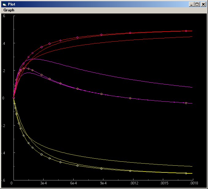
Fig.25
* The simulation mode can be also invoked directly from the "Analysis
- Process Simulation" menu.
10. Wave Separation
SPANA separates the overlapped spectra by using Gauss, Lorentz
or Voigt functions. For example, the procedures in which the spectrum in
the "Overlap.ana" file is separated by Gauss functions is shown below (Fig.26).
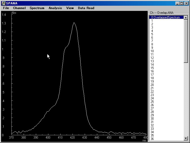 Fig.26 Sample spectrum for wave separation
At first, the Gaussians expected in the spectrum are roughly defined by using the "+" cursor (the "Analysis-Wave Separation-Manual-Gauss" menu). Left click of this cursor leaves a bright point on the screen and the Gaussian (dark green Gaussian in Fig.24) is generated every these 3 bright points (the top and two points showing the half width at half maximum of Gaussian are usually easy to define). The selection whether the generated Gaussian should be used for separation is assigned on the "Wave Set" dialog box, i.e., the "Cancel" button for discard, or the "Set" for the adoption which continues the operation of another definition of Gaussian, or the "OK" which means that the Gaussian is adopted as the final Gaussian component for the calculation (Fig.27).
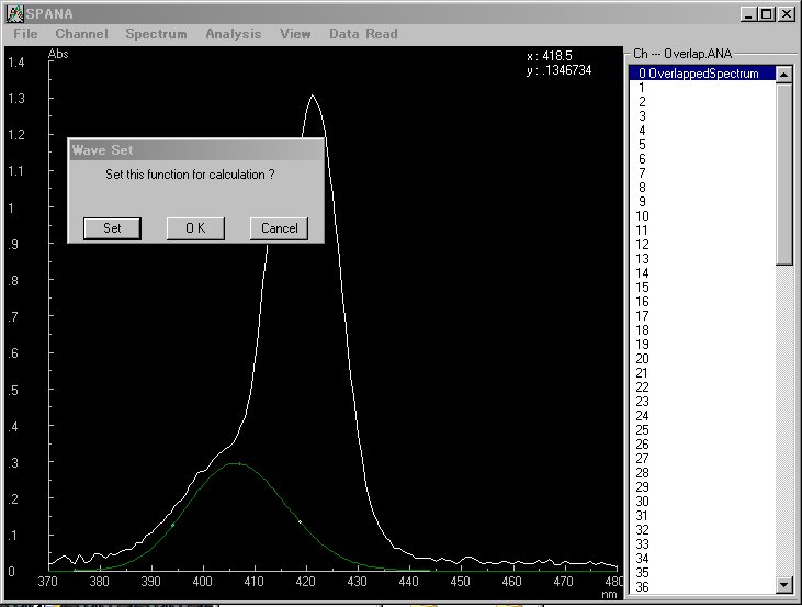
Fig.27 Generation of Gaussian component
After defining all Gaussians (in the present case, 3 Gaussians are defined), the wave length range where the optimization is applied is indicated with the vertical cursor shown on the screen (in this case, 375- 451 nm) and the channels which store the resulting Gaussian components are assigned as usual (Fig.28).
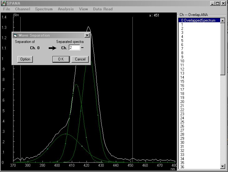
Fig.28 Setting of simulation range
After completion of calculation, the Gaussian components (Gaussian 1-3) and final simulated spectrum are stored in the suggested channels , in this case, Ch. 2-4 and Ch.5, respectively (Fig.29).。
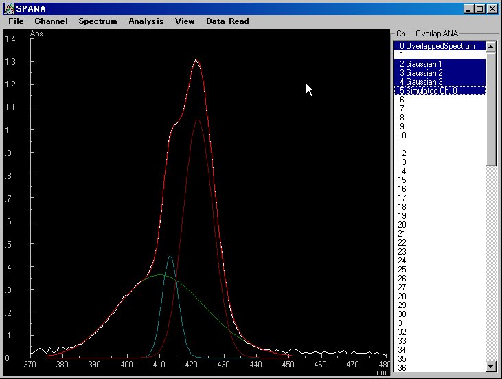
Fig.29 The spectra of original (white), simulated (red), and elemental
Gaussians (dark blue, dark green and dark red)
Note : In the default status, the calculation of the wave separation is performed by using the unit of the wave number, Kcm-1 (alteration is possible). The numerical data for the final Gaussian components are shown in the "Edit" dialog box ("Channel-Channel Edit" menu) as height of top (h), peak position (v Kcm-1), and half width at half height (w Kcm-1) as shown in Fig 30.
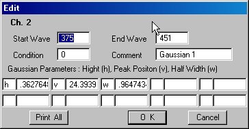
Fig.30 Numerical data for Gaussian in Ch. 2.
11. Analyses of Multicomponent Spectra
If the standard individual spectra of the components contained
in a sample are available, SPANA estimates their compositions in its observed
spectrum. The example is given in the "regression.ana" file which contains 4 standard spectra (Ch. 0-4) and 4 sample spectra
(Ch. 10-13) as shown in Fig.31 and 32.
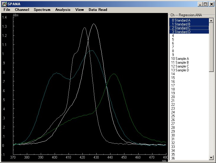
Fig.31 Sample data for regression analysis of multicomponent spectra (standard
spectra).
The regression analyses of SPANA estimates the contents of the standard
spectra in the sample spectra as the form of
Sample X =
a・Standard A + b・Standard B + c・Standard C + d・Standard D eq.7
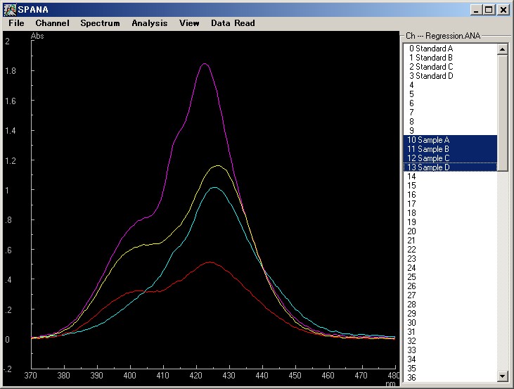
Fig.32 Sample data for regression analysis of multicomponent spectra (sample spectra)
In order to set the conditions for analyses, open the "Regression Analyses" dialog box (the "Analysis-Regression" menu) and set the sample channel (here, "All"), storage channel for the resultant simulated spectra (here, "16-") and the channels of the standard spectra used for the analysis (here, Ch. 0, 1, 2, 3) up to 10 (Fig.33).
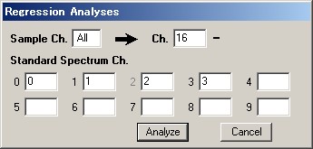 Fig.33
Click of the "Analyze" button start the regression analysis calculation and, then, shows the content coefficients of the standard spectra, a, b, c and d in eq.7, for the sample spectra in the "Result" Table (Fig.34).
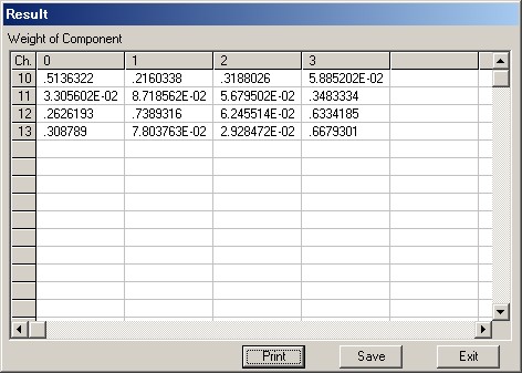 Fig.34
The resultant simulated spectra are stored in the indicated channels (here, Ch. 16-19) as "Composed Ch. X". These composed spectra are shown on the screen as similarly as usual spectrum by "left-click" operation and, furthermore, the component spectra are also shown by "right-click" operation as shown in Fig.35.
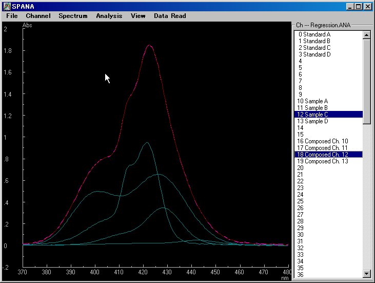
Fig.35 Simulated spectrum (dark red, Ch.18), component spectra (dark blue)
and Sample C spectrum (purple, Ch.12, almost overlapping).
The content coefficients, a, b, c and d, are also recorded in the "Edit" dialog box ( "Channel-Channel Edit" menu) as shown in Fig.36.
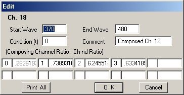 Fig.36
12. 3D View
The "View-3D View" menu opens the new windows for the 3 dimensional
expression of the collected data which has three orthogonal axes of wave
length (x), spectral strength (y), and condition (t or z) variables. The
spectra are shown in the x-y-z 3 dimensional box of which tilt angle and
the size are set in the bottom part of the window. Click of the "Show"
button shows the simple spectra in the box (Fig.37).
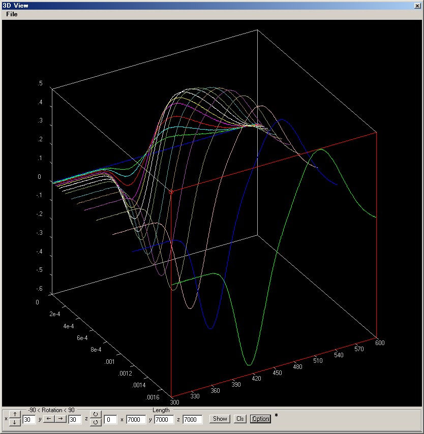
Fig. 37 Surface-None, Color Separation-Channel
Other types of 3D graphs such as the spectral surface with mesh representation, the contour map, and the spectral screens may be shown by setting the necessary parameters in the "Option" dialog box (Fig.38 and 39).
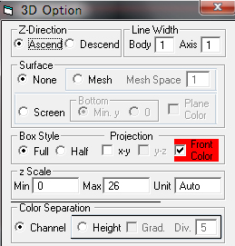
Fig.38
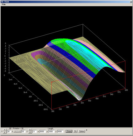
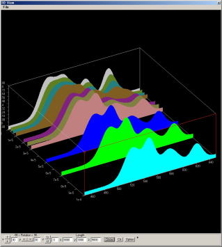
Fig.39 Left: Surface-Mesh, Color Separation-Height , Right: Surface-Screen,
13. Analyses of NMR Data
a) Titration
For chemical exchange-equilibrium which is rapid on the NMR time-scale,
ABi-1 + B <-> ABi i = 1 - n
the individual observed chemical shift δobs is the mole-fraction-weighted average of the shifts δ for the corresponding
nuclei in chemical species ABi existing in the system.
δobs = ΣPABi δABi
Here,
PABi = [ABi] / [A]Total , [A]Total = Σ[ABi] , i = 0 - n.
then, the change of the chemical shift, Δδobs, is
Δδobs = δobs - δA = Σ(ΔδABi/[A]Total)[ABi] , ΔδABi = δABi - δA, i = 1- n
Since, regarding ΔδX/[A]Total as ΔεX , the relationship between the observed values and the concentrations is
the same as that for the electronic spectrum, the optimization models of
SPANA are also applicable for this type of NMR titration data.
The analysis is performed for the chemical shift data which are set in
the "Result" table by using the numerical key-board or by reading
the data file of the ".lsq" format.
Following is the example of analysis for the data of the attached sample
file, "NMR1-2.lsq", containing two chemical-shift change data
(y1 and y2) vs. ligand concentration (t) for a 1:2 complex formation system
(Fig.40).
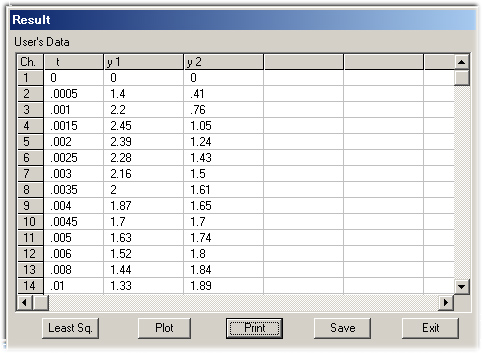 Fig.40
The optimization by using the 1:2 sequential complex formation model results in the following parameters (Fig.41),
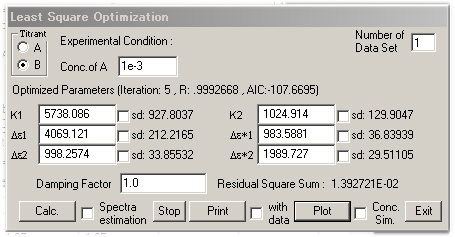 Fig.41
K1 = 5.7 x 10³, K2 = 1.0 x 10³, Δδ1AB = 4.1 (Δε1 x [A]Total), Δδ1AB2 = 0.98 (Δε*1 x [A]Total), Δδ2AB = 1.0 (Δε2 x [A]Total), Δδ2AB2 = 2.0 (Δε*2 x [A]Total) (Fig.41)
b) NMR Line Shape Fitting
The 1H-NMR signal shape, I(ν), under the equilibrium, A <-> A', is theoretically
determined as the function containing the following 7 parameters,3)
νA : chemical shift of A , νA' : chemical shift of A' , PA : mole-fraction of A , kA : rate constant for A -> A'
T2A : spin-spin relxation time of A , T2A' : spin-spin relaxation time of A' , C : normalization factor
The NMR line shape fitting method of SPANA (Fig. 42) optimizes these 7
parameters to minimize the residual square sum between the theoretical
and observed signal shapes.
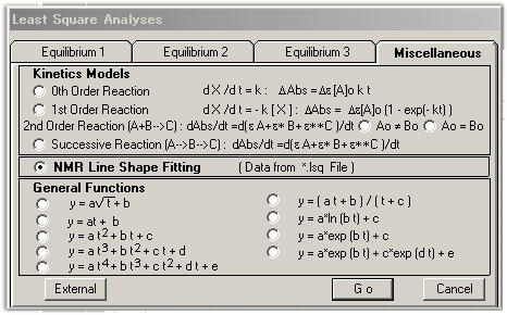 Fig.42
The results of analysis for the attached sample data, nmrfit-spana.lsq,
by the "NMR Line Shape Fitting" model is shown below (Fig.43).
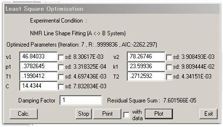 Fig.43
The "Plot" command shows the graphics of the theoretical-observed data fitting (Fig.44).
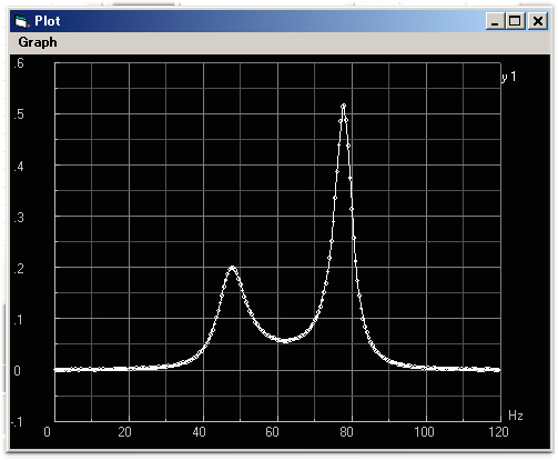 Fig.44
14. Analyses of Concentration Data
Since the absorbance of the electronic spectrum is linearly proportional
to the concentration of the corresponding chemical species under the Lambert-Beer
Law conditions, specifying 1.0 for the proportionality constant, the absorbance
term means the concentration. Thus, the data for the concentration of individual
chemical species in the system can be analyzed by SPANA using this relationship.
For example, the analysis of the successive reaction, A -> B -> C,
using concentration data is shown below.
The attached data, "Series.lsq", contains following two data
sets of the concentrations of A, B and C (y1, y2, y3) vs. time (t) observed
for different initial concentrations [A]0 (Fig.44),
{ Ch.1-5 : t = 0.1-1.5 , [A]0 = 101.53 } and { Ch.6-13 : t = 0.15-2.1 , [A]0 = 200.1 }:.
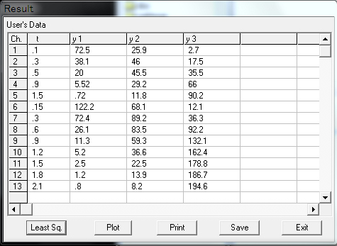 Fig.44
In order to analyze these data in concentration mode, following parameter
settings are applied to the "Least Square Analyses - Miscellaneous
Model - Successive Reaction" dialog box (Fig.45).
Since y1 means [A] which is related to the absorbance term according to
the equation of
Absobs = ε1[A] + ε*1[B] + ε**1[C],
the values of <ε1, ε*1, ε**1> for y1 are fixed to <1, 0, 0>. In the same way, those for y2
an y3 are fixed to <0, 1, 0> and <0, 0, 1>, respectively. The check-boxes for all these parameters are checked to remove from optimization calculation.
Setting two initial concentrations of A and the initial guess values for k1 and k2, the optimization gives
the results shown in Fig.45.
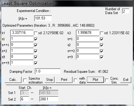 Fig.45
The "Plot" command shows the fitting graph of Fig.46.
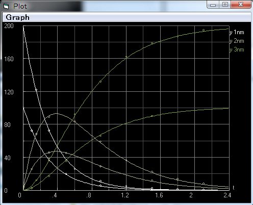 Fig.46
15. Least Square analyses for User's Function (Ver.5 Only) 4)
Although the procedures of the least square analyses for the user's function
may be different according to the user's situation, the outlines of the
analyses are described below, as an example, by using the sample data, "titrn283-323.ana" (for the program of the analyses, see the "Analyses" page).
The file, titrn283-323.ana, contains the following temperature dependent
spectroscopic titration data.
| Data Set No. | 1 | 2 | 3 | 4 | 5 |
| Ch. | 200-209 | 215-224 | 230-240 | 245-254 | 260-270 |
| Temp (K) | 283 | 293 | 303 | 313 | 323 |
| Conc. [A] (M) | 1.0 x 10⁻⁵ | 0.83 x 10⁻⁵ | 1.0 x 10⁻⁵ | 1.15 x 10⁻⁵ | 0.91 x 10⁻⁵ |
| Conc. [B] (M) | 0 - 5 x 10⁻⁵ | 0 - 1 x 10⁻⁴ | 0 - 2 x 10⁻⁴ | 0 - 5 x 10⁻⁴ | 0 - 1 x 10⁻³ |
The different spectra of this data are shown in Fig. 47.
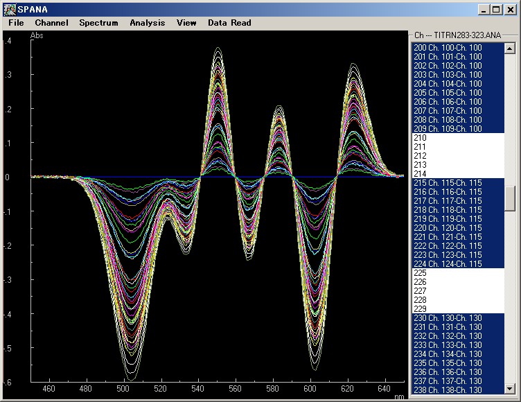
Fig.47
Collecting necessary data, click of the "External" button in the "Miscellaneous Models" page (Fig.40) of "Least Square Analyses" dialog box shows the "External Least Square Program" dialog box (Fig.48).
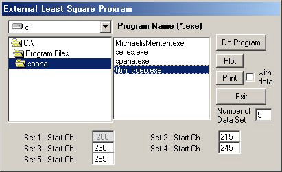 Fig.48
If the data contain two or more data sets, set the number of data set and the top channel of each set, select the user's program "titrn_t-dep.exe", for example, and click the "Do Program" button. The program read the "spana_lsq.dta" file and open new MS-DOS WINDOW. According to request of the program, set the necessary data such as the number of parameters, p[i], and constants, c[i], and initial guess of p[i], then the results of calculation are shown as Fig.49
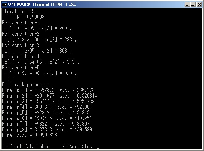
Fig.49
After calculation, this program may generate the data for graphic simulation on user's request, which are used for theoretical simulation curves by clicking the "Plot" button in Fig.41to show the simulation graphs Fig.50.
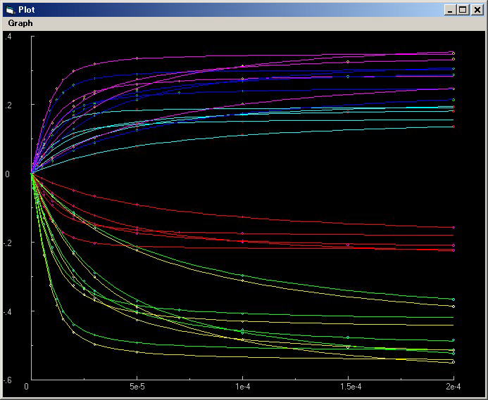
Fig.50
References.
1) For example of the nonlinear least square calculation,
a) S. L. S Jacoby, J. S. Kowalik, J. T. Pizzo,
"Interative Methods for Nonlinear Optimization Problems", Prentice
Hall, Inc., N.J, 1972.
b) T. Nakagawa and Y. Koyanagi, "Analyses
of Experimental Data by Least Square Method (Japanese)" (UP Applied
Mathematics Series 7), University of Tokyo Press, Tokyo, 1982.
2) For example of regression analyses and wave separation,
a) D. J. Leggett, "Numerical Analysis of Multicomponent
Spectra", Analytical Chemistry, vol.49, 276, 1977
b) R. D. B. Frasher, E. Suzuki, "Resolution
of Overlapping Absorption Bands by Least Squares Procedures", Analytical
Chemistry, vol. 38, 1770, 1966.
c) S. Minami, Ed., "Treatment of Wave Data
in Scientific Measurement (Japanese)", CQ Press Inc. (Japan), Tokyo,
1986 and references therein.
3) J. Sandstroem, "Dynamic NMR Spectroscopy.", Academic Press,
1982
4) For details of this section, contact to my e-mail address.