analyses-e

1. Equilibrium and Reaction Rate Analyses

SPANA performs the equilibrium or rate analyses for the titration data or time course data by using the non-linear least square optimization procedure.
The calculation minimizes the residual square sum value (ss) to optimize the parameters such as the equilibrium constants, rate constants and absorptivities. The ss value is evaluated from the observed strengths of spectra (Y_obs) and the theoretical ones (Y_theoretical) calculated by using the parameters and independent experimental variable such as concentrations, temperature and/or time, as follows.
　　　　　　　　　　　　　　　　　　　ss = ∑（Yobs - Ytheoretical)^2

SPANA provides the following equilibrium and rate models.

Model	Theoretical Spectral Strength
Equilibrium Model
Sequential 1:n Complex formationl AB_i-1 + B <-> AB_i ,　　　 K_i= [AB_i]/[AB_i-1][B] 　i = 1～n , n_max = 5	Abs = ε_A[A] + ∑ε_ABi[AB_i]
Sequential 1:n Complex formation accompaning Pre-equilibrium of A pA* <-> qA,　　　　　　　　　K_o= [A]^q / [A*]^p AB_i-1 + B <-> AB_i ,　　　 K_i= [AB_i]/[AB_i-1][B] 　i = 1～n , n_max = 5	Abs = ε_A[A] + ε_A[A] + ∑ε_ABi[AB_i]
Independent 1:n Complex formation A^{empty i} B_j-1 + B <-> A^{occupied i} B_j　　　　K_i = [A^{occupied i} B_j]/[A^{empty i} B_j-1][B] 　i , j = 1～n , n_max = 5	Abs = (∑ε_A)[A] + ∑( ∑_{_empty}ε_A + ∑_{_occupied}ε_AⁱB)[AB_j]
pH titration model with n pKa’s AH_i-1 + H⁺ <-> AH_i 　　　K_i= [AH_i]/[AH_i-1][H⁺]　　i = 1～n , n_max = 5	Abs = ε_A[A] + ∑ε_AHi [AH_i]
n-Step 1 : n Complex formation AB_i-1 + B <-> AB_i 　K=[AB_i]/[AB_i-1][B]^a (i = 1～n) 　（a=1 : Independent complexation 　（a>1 : Cooperative complexation　<Hill’s type expression>） - Job's Analyses - 　[A]_Total + [B]_Total = C (constant) 　φ = [B]_Total / C , 1 - φ = [A]_Total/ C , φ= 0 ～1	Abs = nε_A[A] + ∑{(n - i)ε_A + iε_AB}(n ! / ((n - i) !・i !)) [AB_i]
One-step m:n Complex formation mA + nB <-> A_mB_n 　　　K = [A_mB_n]/[A]^m[B]ⁿ - Job's Analyses - 　[A]_Total + [B]_Total = C (constant) 　φ = [B]_Total / C , 1 - φ = [A]_Total/ C , φ= 0 ～1	Abs = ε_A[A] + ε_AmBn[A_mB_n]
One-step m-n Self-reorganizaton mA <-> nA* 　　　K = [A*]ⁿ/[A]^m	Abs = ε_A[A] + ε_A[A]
Thermal Dependency mA<-> nA* 　　K = [A*]ⁿ/[A]^m = exp(-(ΔH-TΔS)/RT) A + B <-> AB K = [AB]/[A][B] = exp(-(ΔH-TΔS)/RT)	Abs = ε_A[A] + ε_A[A] Abs = ε_A[A] + ε_AB[AB]
Competitive 1:1 Complex formation 　A + I <-> AI　　　K₀ = [AI]/[A][I] 　A + B <-> AB　　K₁ = [AB]/[A][B] 　　　A, B : spectroscopically inactive 　　　　　I : spectroscopically active	Abs = ε_I [I] + ε_AI [AI]
Competitive 1:2 Complex formation 　A + I <-> AI　　　　　K₀ = [AI]/[A][I] 　A + B <-> AB　　　　K₁ = [AB]/[A][B] 　AB + B <-> BAB　　K₂ = [BAB]/[AB][B] 　　　A, B : spectroscopically inactive 　　　　　I : spectroscopically active	Abs = ε_I [I] + ε_AI [AI]
Reaction Rate Model
0 th Oder reaction	Abs = k t +Abs₀
1st Order reaction A → B 　k : rate const.	Abs = ε_A[A]t + ε_B[B]t
2nd Order Reaction A + B → C　k : rate const.	Abs = ε_A[A]t + ε_B[B]t + ε_C[C]t
Successive Reaction A → B → C　k₁, k₂ : rate const.	Abs = ε_A[A]t + ε_B[B]t + ε_C[C]t
NMR Line Shape Analyses A <-> B　　　k₊ , k_- : rate const.	I(v) = f (v, v_A, v_B, p_A, k₊, T_2A, T_2B, C)
General Function y : dependent variable t : independent variable a, b, c, d, e, f : parameters to be optimized	y = a √ t + b 　y = a t + b 　y = a t² + b t + c 　y = a t³ + b t² + c t + d 　y = a t⁴ + b t³ + c t² + d t + e 　y = a t⁵ + b t⁴ + c t³ + d t² + e t + f 　y = (a t + b) / (t + c) + dt 　y = a ln (b t) + c t + d 　y = a exp (b t) + c t + d 　y = a exp (b t) + c exp (d t) + e 　y = a / (1 + exp (-(t - b) /c) + d t + e (Logistic function) 　y = a / (1 + (t - b)²/c²) + d t + e (Lorentz function) 　y = a exp (-(t - b)²/c²) +d t + e (Gauss function)
User's Function y[i] : dependent variable x[1] : independent variable ( = t) c[i] : constant defined in the program p[i] : parameters to be optimized	y[i] = f ( x[1], c[i], p[i] )

2. Wave Separation

SPANA perform wave separation using Gauss, Lorentz, and Voigt functions. The type and number of the wave components are set by the user.

3. Component analyses

SPANA estimates the contents of the standard spectra of components (max. 10) in the observed spectra by the method of multiple regression analysis.

4. Least Square Analyses for User's Functions

The least square analyses for user defining functions are available. The following are the outline of preparation of the program which can be used in SPANA (for the practical procedures of the analyses, see "Example" page).

a) The Data
SPANA produces the text file, spana_lsq..dta, containing the collected spectral data in the spana folder. The file format is shown below.

Format of "spana_lsq.dta" file
　　 sp : number of sampling point, ds : number of data set, d(i) [ i = 1 - ds ] : number of data for i^th data set
　　y(j) : spectral strength , t : condition value,

b) The Program
SPANA analyses the collected data by using the programs which read the spana_lsq.dta file. For this purpose, the general least square analyses programs written in C language, spana_lsq.c, is provided in the version 5.
The user prepares C-source file in which the function describing the user's system is defined, links it with spana_lsq.c, and compiles to make the execute program of the ".exe" type, which may be called from SPANA directly. For compilation of the programs, not only commercial C compilers but also free one such as DJGPP and Micosoft Visual Studio C++ are available.

The following variables, parameters, and constants are defined ;
　　y[i] : dependent variables (ex. Abs in the titration experiment), i = 1 - 20
　　x[i] : independent variable (ex. titrant concentration), i = 1 (fixed in SPANA)
　　c[i] : constants (ex. sample concentration), i = 1 - 30
　　p[i] : optimized parameters (ex. equilibrium constants, molar absorption constants), i = 1 - 20

By using these symbols, the functions of user's system, y[i] = f (x[i] , c[i] , p[i] ), are defined in the C-source as
　　　void function( int i, double x[], double y[])
　　　　　｛　　　　　　　　　　　　　　　　　　　　　　　　　　｝
(where i is number of dependent variables).

The following program is that applicable for determination of thermodynamic parameters, ΔH and ΔS. by using temperature dependent spectral titration data of the 1:1 complex formation system at 10 different wave length position.

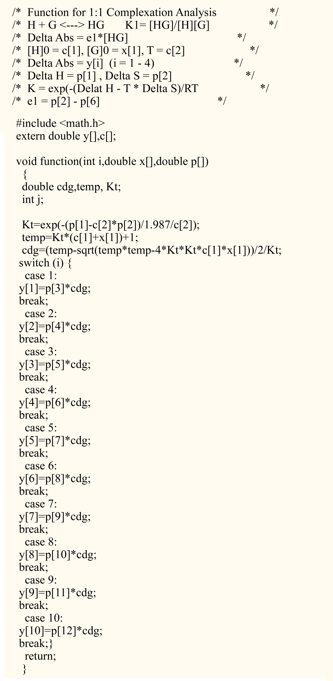
In this source program, the lines between /* and */ are comments and the following part defines the difference absorption,
　　ΔAbs = (Abs - ε_A[A] ₀ =) Δε[AB].
After saving this file, for example, as the name of "titrn_t-dep.c", the execution program, titrn_t-dep.exe, is obtained by linking with "spana_lsq.c" and compiling the source programs as follows,
　　gcc -o titrn_t-dep.exe spana_lsq.c titrn_t-dep.c, for DJGPP
or
　　cl titrn_t-dep.c spana_lsq.c, for Visual Studio C++

SPANA ver.5 provide another least square program for the analysis of the reaction kinetics, spana_redap.c, which analyses the time dependent spectral change by numerical integration of differential equations for chemical reactions without using the integral forms. For the detail of this program, contact me by e-mail.